Lennard-Jones Potential in Molecular Dynamics

Understanding Lennard-Jones Potential

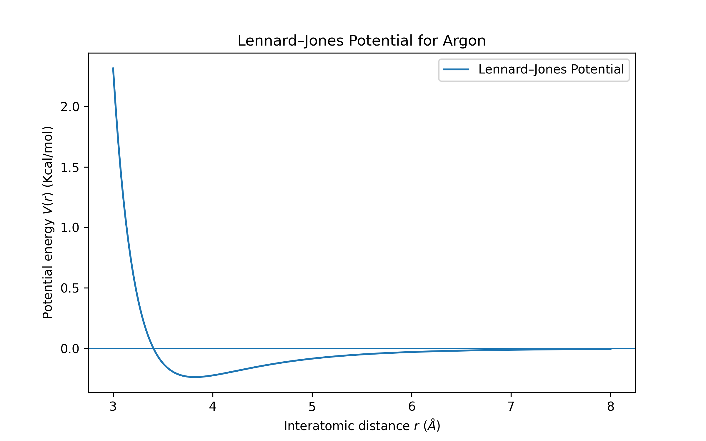
Molecular dynamics simulations rely on interatomic potentials to describe particle interactions. One of the most common is the Lennard-Jones (LJ) potential, which accounts for both repulsion and attraction between atoms. \[ V(r) = 4 \, \epsilon \underbrace{\left(\frac{\sigma}{r}\right)^{12}}_{\text{repulsion}} - 4 \, \epsilon \underbrace{\left(\frac{\sigma}{r}\right)^6}_{\text{attraction}} \] Here, \(\sigma\) is the distance where the potential crosses zero, and \(\epsilon\) is the depth of the potential well. The \((\sigma/r)^{12}\) term models repulsion, and the \((\sigma/r)^6\) term models attraction.

Repulsion: Pauli Exclusion Principle

When two atoms approach each other, their electron clouds overlap. According to the Pauli exclusion principle, electrons cannot share the same quantum state. Some electrons are forced into higher energy levels, increasing potential energy. The gradient of this energy produces a repulsive force, preventing atomic collapse.

Attraction: Van Der Waals Forces

Even neutral atoms can experience weak attraction via instantaneous dipoles. An atom's temporary dipole can induce a dipole in a neighbor, resulting in a fluctuating Coulomb interaction. Macroscopically, the sum of these interactions manifests as van der Waals forces.

How LAMMPS Gets the Trajectory

First, we need to specify the position of each atom. The distance between two atoms is \(r\), which is used to determine the potential. The force is the negative gradient of the potential: \[ \mathbf{F} = -\nabla V(\mathbf{r}) \] Using this force we get acceleration: \[\mathbf{a} = \mathbf{F}/m\]

Force and Velocity-Verlet Algorithm

LAMMPS updates particle positions and velocities using the velocity-Verlet algorithm: \[ \mathbf{r}(t+\Delta t) = \mathbf{r}(t) + \mathbf{v}(t) \Delta t + \frac{1}{2} \frac{\mathbf{F}(t)}{m} \Delta t^2 \] \[ \mathbf{v}(t+\Delta t) = \mathbf{v}(t) + \frac{1}{2} \left[ \frac{\mathbf{F}(t)}{m} + \frac{\mathbf{F}(t+\Delta t)}{m} \right] \Delta t \] This ensures positions and velocities are updated accurately at each timestep.

Example: Two-Atom 1D Simulation

Consider two argon atoms in 1D with initial positions \(x_1=1.5\) Å, \(x_2=5.5\) Å, and velocities \(v_1=v_2=0\). Using LJ parameters \(\sigma=3.4\) Å, \(\epsilon=0.238\) kcal/mol, and a small timestep \(\Delta t = 1\) fs, LAMMPS calculates forces and updates positions iteratively. Over time, atoms oscillate due to attraction and repulsion.