Maxwell–Boltzmann Velocity Distribution for LAMMPS

What is the Maxwell–Boltzmann Distribution?

Imagine placing a bunch of particles inside a box and fixing the temperature. Even then, you will never find all particles moving with the same speed. Some are slow, some are extremely fast, but most of them hover around a typical value.

This simple idea, when treated properly using classical statistical mechanics, leads to what we call the Maxwell–Boltzmann (MB) velocity distribution. It describes how particle speeds are distributed when the system is in thermal equilibrium. The key point is that the distribution depends only on the particle mass and the temperature.

For a three-dimensional system, the probability density of finding a particle with speed \(v\) is

\[ f(v) = 4\pi \left( \frac{m}{2\pi k_B T} \right)^{3/2} v^2 \cdot \exp(-\frac{m v^2}{2 k_B T}) \]

Here, \(m\) is the particle mass, \(T\) is the temperature, and \(k_B\) is the Boltzmann constant.

Understanding the Shape of the MB Curve

Below is the Maxwell–Boltzmann curve plotted using SI units with \(m = 6.63\times10^{-26}\,\text{kg}\), \(k_B = 1.38\times10^{-23}\,\text{J/K}\), and \(T = 300\,\text{K}\).

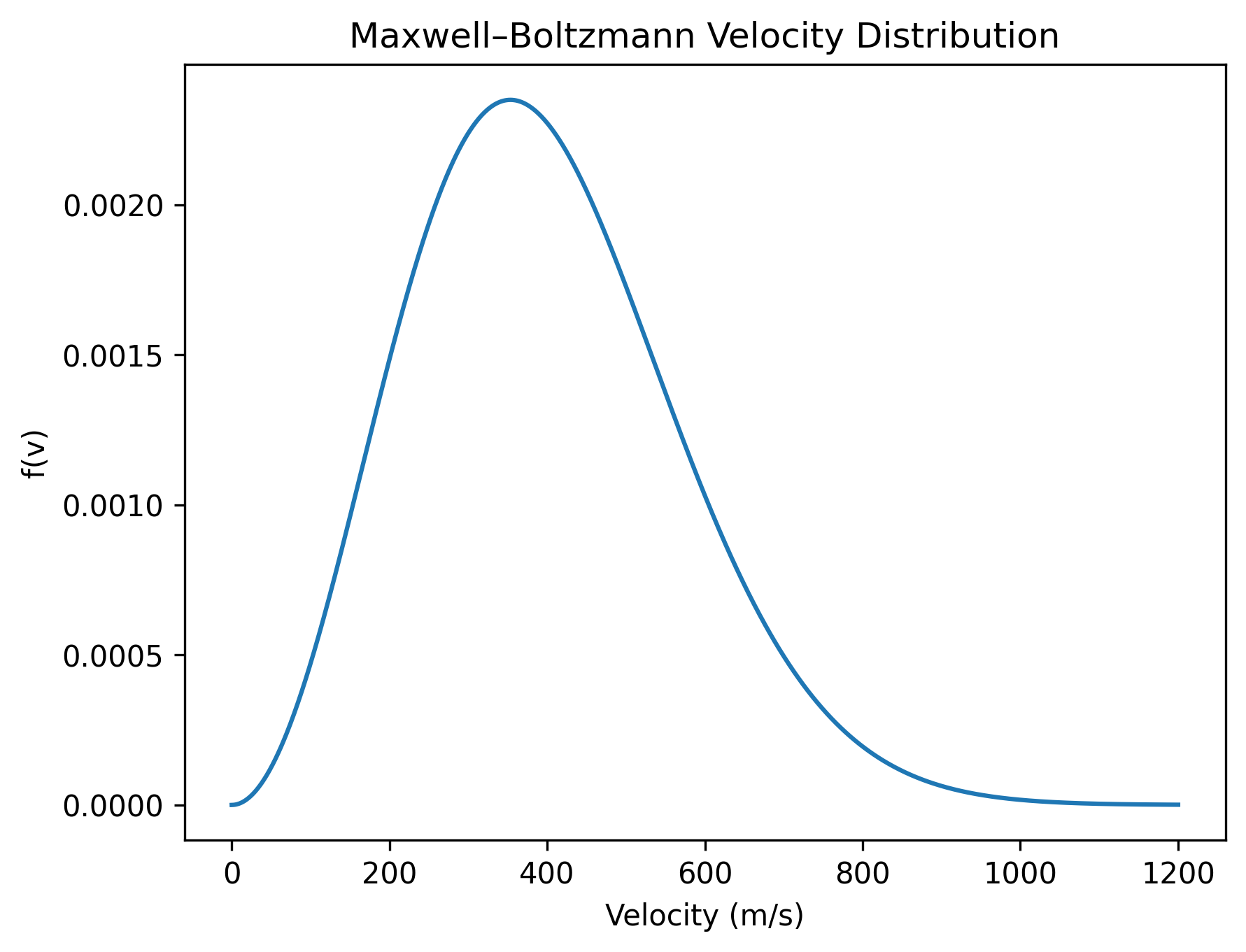
The curve is clearly asymmetric. The peak corresponds to the most probable speed — the speed that the largest number of particles have.

To see where this shape comes from, ignore the constants and focus only on the structure of the equation:

\[ f(v) \propto v^2 e^{-v^2} \]

At very low velocities, the \(v^2\) term dominates and suppresses small speeds. At very high velocities, the exponential term takes over and rapidly kills the probability. The competition between these two effects produces the characteristic MB curve.

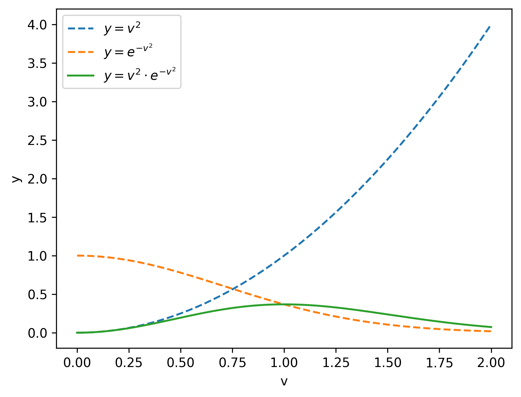
So low velocities are suppressed by the \(v^2\) factor, while high velocities are suppressed exponentially due to thermal energy limits.

Effect of Temperature

Increasing the temperature shifts the peak of the distribution to the right and makes the curve broader. Higher temperature simply means higher average kinetic energy, so particles explore larger speeds.

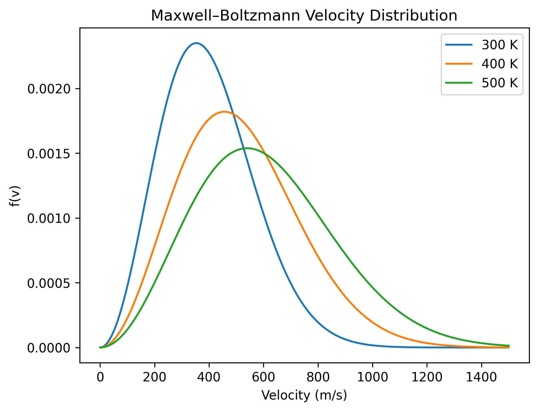
One important thing never changes: the area under each curve remains the same. Regardless of temperature, the total probability must always be 1.

LAMMPS Velocity

Using LAMMPS, we can extract the velocities in the x, y, and z directions from a dump file. By processing this data, we can calculate the speed of each particle: \[ v = \sqrt{v_x^2 + v_y^2 + v_z^2} \] and plot a histogram showing how many particles fall within small velocity ranges.

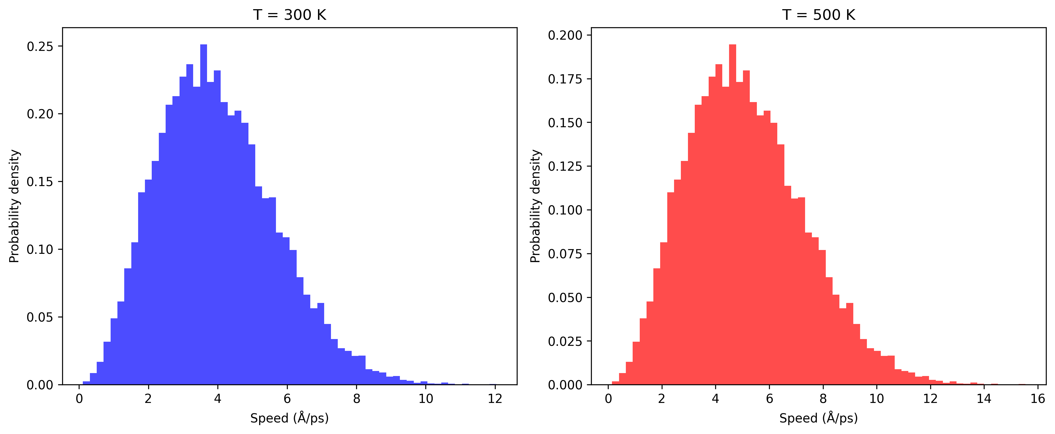
From the plot, we can see that the histograms at 300 K and 500 K both follow the Maxwell–Boltzmann theoretical distribution closely. Increasing the temperature shifts the most probable velocity to the right, as expected.

Overlaying the histogram with the theoretical MB curve using the same mass and temperature shows a strong agreement, confirming that the simulation is thermally equilibrated.

All the essential code (LAMMPS and python) are available at github