Morse Potential

Understanding Morse Potential

In molecular dynamics simulations, interatomic potentials define how atoms influence one another. The Lennard–Jones potential is adequate for noble gases, where no true chemical bonding occurs. However, modeling real chemical bonds demands a more physically accurate description.

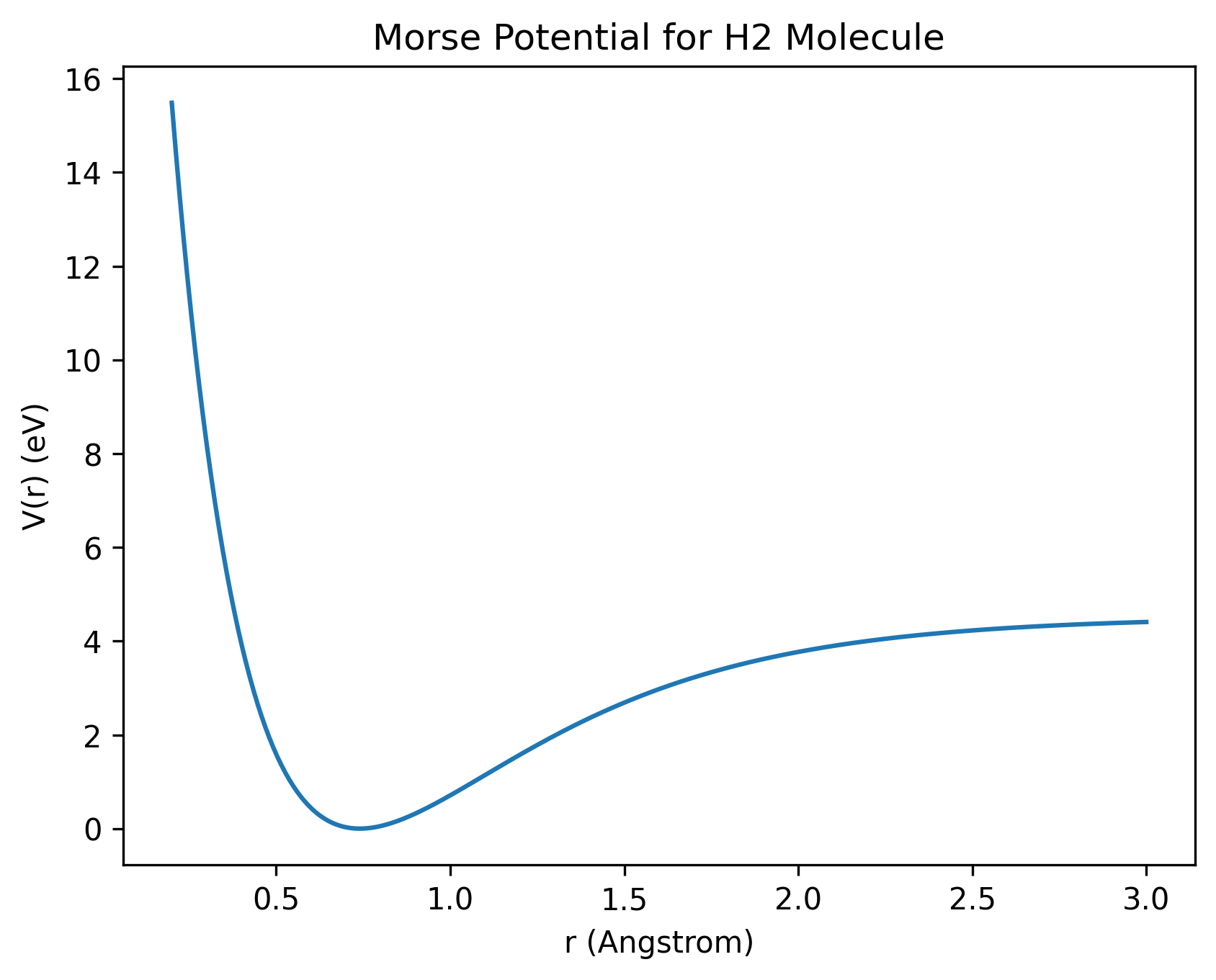
The Morse potential models chemical bonds more realistically, including how they stretch and eventually break. Here, a bond can be thought of as a spring connecting two atoms. \[ V(r) = D_e \bigl( 1 - e^{-a(r - r_e)} \bigr)^2 \]

Physical Meaning of Parameters

The parameter r_e represents the equilibrium bond distance, meaning the spring is at its natural length — neither stretched nor compressed.

The parameter a controls the stiffness of the bond, similar to how thick or thin (hard or soft) a spring is. A higher value of a means a stiffer spring, so the force increases rapidly when the atoms move away from equilibrium. A lower value of a means a softer spring, and the force increases more gradually.

Here, D_e is the bond dissociation energy. It represents the energy required to break the spring — that is, to completely separate the two atoms.

Bond Formation and Anharmonicity

Real chemical bonds are anharmonic. Near equilibrium, the Morse potential behaves approximately like a harmonic spring: \[ V(r) \approx \frac{1}{2} k (r - r_e)^2 \] But unlike a simple harmonic oscillator, the Morse potential becomes asymmetric. Stretching the bond weakens it gradually, while compression increases energy sharply. This asymmetry correctly models bond breaking.

All the code for this simulation is available at GitHub.