Simulating Quantum Measurement: Probability vs. Observation
In quantum mechanics, few ideas capture the imagination quite like the measurement problem. A quantum system before measurement can exist in an elegant linear superposition described by continuous complex probability amplitudes. Yet, whenever we perform an observation, the system yields a single discrete eigenvalue—either a $0$ or a $1$.
As an undergraduate physics student working at the intersection of computational physics and scientific computing, I wanted to understand this transition deeply from first principles: How do repeated, discrete measurements accumulate into continuous Born-rule probabilities? How do finite-sample statistical fluctuations behave, and how fast do they decay as we increase the number of measurement shots?
To explore this rigorously, I developed an open-source numerical simulation from scratch in Python: quantum-measurement-simulation. This blog shares how the simulation works, the mathematics governing it, and what the numerical experiments reveal.
Part 1: The Physics & Mathematical Model
Let us consider a pure single-qubit quantum state written in the standard computational basis $\{|0\rangle, |1\rangle\}$:
For $|\psi\rangle$ to represent a physically valid state, it must satisfy the normalization condition:
According to the Born rule, when we measure $|\psi\rangle$ in the computational basis, the probability of obtaining outcome $0$ or outcome $1$ is given by the squared magnitude of their respective amplitudes:
In an ideal quantum experiment, each measurement is an independent, identically distributed Bernoulli trial. If we prepare the exact same state $|\psi\rangle$ and measure it $N$ times independently:
- The count $K$ of measuring outcome $1$ follows a Binomial distribution: $K \sim \mathrm{Binomial}(N, p)$, where $p = P(1) = |\beta|^2$.
- The empirical sample frequency is $\hat{p}_N = \frac{K}{N}$.
- The theoretical expectation is $\mathbb{E}[\hat{p}_N] = p$.
- The theoretical standard error of the observed frequency scales as:
$$\mathrm{SE} = \sqrt{\frac{p(1-p)}{N}}$$
Part 2: Building the Simulation Engine
Rather than relying on heavy quantum framework packages, I designed a modular, clean Python architecture from first principles:
QuantumState: Stores complex amplitudes $\alpha$ and $\beta$. Crucially, it rejects non-normalized states within a numerical tolerance of $10^{-9}$—no silent normalization is allowed, ensuring physical honesty.measure_state: Simulates projective computational-basis measurements using an isolated NumPyGenerator(PCG64) for exact reproducibility.statistics: Computes occurrence counts, observed frequencies, absolute deviations, and root-mean-square errors ($\mathrm{RMSE}$) across ensembles.
The core measurement sampling logic in Python is concise and clean:
import numpy as np

def measure_state(state, shots, rng=None, seed=None):
    if rng is None:
        rng = np.random.default_rng(seed)

    # Born-rule theoretical probabilities
    probabilities = [state.prob_0, state.prob_1]

    # Sample binary outcomes strictly restricted to {0, 1}
    outcomes = rng.choice([0, 1], size=shots, p=probabilities)
    return outcomes
Part 3: Numerical Experiments & Results
To systematically test our theoretical expectations, we execute three distinct numerical experiments.
Experiment A: Measurement Distribution ($N = 1{,}000$ Shots)
We prepare a balanced superposition state:
Simulating $1{,}000$ shots with a fixed random seed yields the following distribution:
| Outcome | Simulated Count | Observed Frequency | Theoretical $P(x)$ | Absolute Deviation |
|---|---|---|---|---|
| $|0\rangle$ | 503 | 0.5030 | 0.5000 | 0.0030 |
| $|1\rangle$ | 497 | 0.4970 | 0.5000 | 0.0030 |
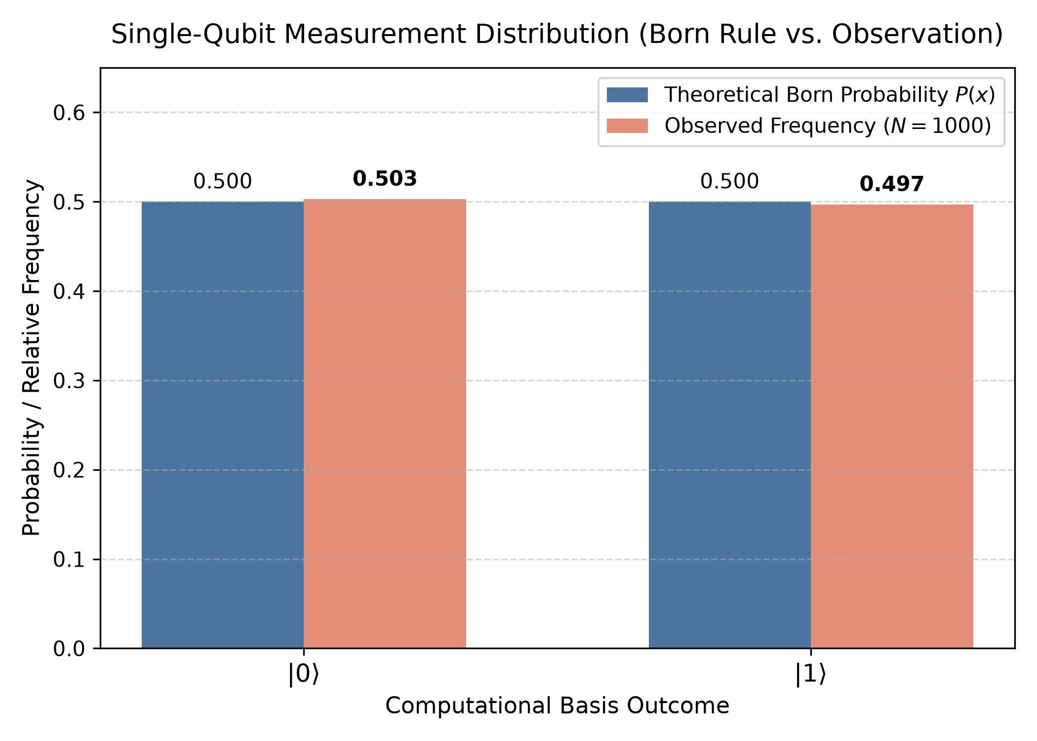
The absolute deviation of $0.0030$ is well within the theoretical standard error expected for $1{,}000$ shots ($\mathrm{SE} = \sqrt{0.5 \times 0.5 / 1000} \approx 0.0158$).
Experiment B: Cumulative Frequency Convergence ($N = 10{,}000$ Shots)
Next, we track the running cumulative frequency $f_n(1) = \frac{1}{n}\sum_{i=1}^n x_i$ as a stream of $10{,}000$ shots are measured on the balanced superposition state:
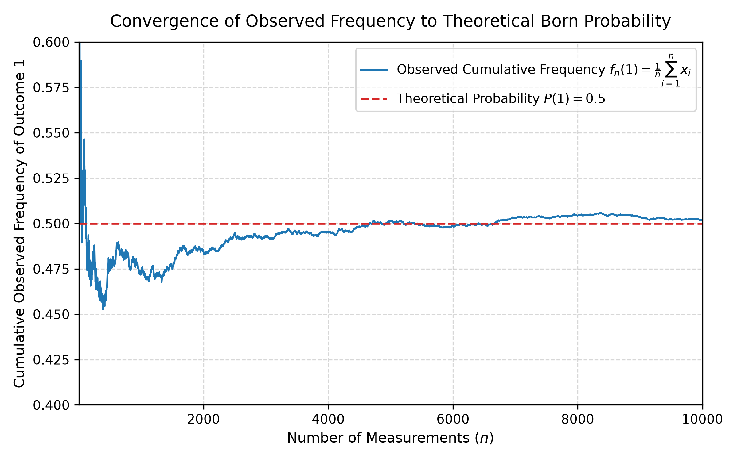
Notice how the curve behaves across different sample sizes:
- Low-sample regime ($n < 500$): The observed frequency fluctuates wildly, swinging between $0.45$ and $0.59$. A small sample does not guarantee the theoretical probability!
- Asymptotic stabilization: As $n$ grows past several thousand shots, the fluctuations dampen, centering tightly around $0.5$.
- Non-monotonic convergence: The curve does not approach $0.5$ as a smooth monotonic line; it naturally oscillates above and below the theoretical line, showing the genuine random nature governed by the Law of Large Numbers. At $n = 10{,}000$, the final observed frequency is $0.5019$.
Experiment C: Statistical Scaling Law ($1/\sqrt{N}$)
To rigorously test the scaling of empirical precision, we simulated experiments across four orders of magnitude: $N \in \{10, 100, 1{,}000, 10{,}000\}$. For each sample size, we performed $M = 500$ independent simulated experiments and computed the empirical root-mean-square error ($\mathrm{RMSE}$):
| Sample Size ($N$) | Theoretical $\mathrm{SE}$ | Simulated $\mathrm{RMSE}$ ($M=500$) | Ratio ($\mathrm{RMSE} / \mathrm{SE}$) |
|---|---|---|---|
| 10 | 0.15811 | 0.14799 | 0.9359 |
| 100 | 0.05000 | 0.04714 | 0.9429 |
| 1,000 | 0.01581 | 0.01604 | 1.0147 |
| 10,000 | 0.00500 | 0.00494 | 0.9871 |
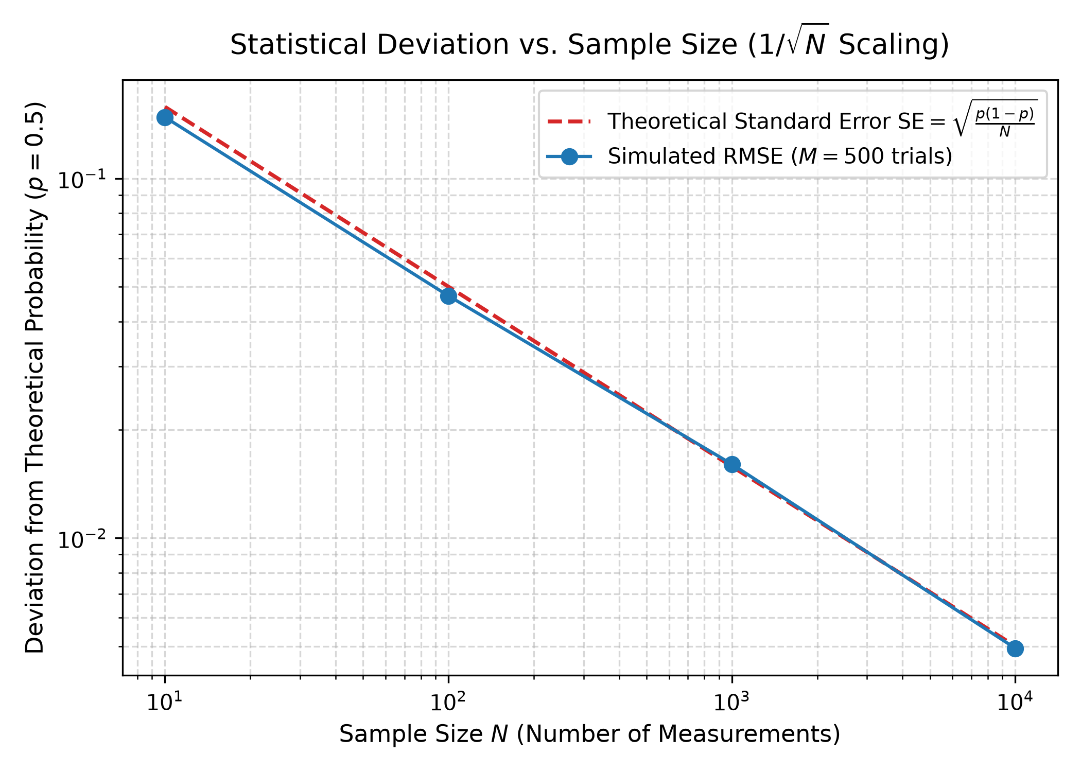
Plotting this on a log-log scale produces an almost perfect linear fit with slope $-1/2$. Every $10\times$ increase in sample size reduces empirical uncertainty by a factor of $\sqrt{10} \approx 3.16$. This confirms that finite-sample quantum measurement errors strictly follow standard statistical mechanics.
Part 4: Scientific Boundaries & Takeaways
While building and testing this simulation, it was important to maintain clear scientific boundaries:
- Classical simulation vs. quantum hardware: This project models ideal Born-rule measurement statistics using classical pseudo-random number generators. It does not interface with physical superconducting or trapped-ion qubits.
- Randomness alone is not quantum: Classical coin tosses follow the exact same binomial distribution and $1/\sqrt{N}$ scaling. The uniqueness of quantum mechanics lies in superposition and interference, whereas the measurement act itself connects to classical probability.
- Idealized model: Real-world quantum computers suffer from state preparation and measurement (SPAM) errors, detector crosstalk, and environmental decoherence.
Source code, experiment scripts, and unit tests are fully open source and available on GitHub:
👉 https://github.com/azam-alif/quantum-measurement-simulation
Feel free to clone the repository, run the experiments, and test different quantum states!